
Brief Introduction:The Antarctic is one of the cold sources of the Earth's atmosphere and a region that is sensitive to climate change. With global warming, Antarctica has become a key area for international programs to study global climate change. Most of the world's ice and snow is stored in the Antarctic, and more than 95% of Antarctica is covered by ice sheets with an average thickness of 2,000 meters, ice shelves and snow that is not covered all year round. It has an ice continent that can raise the global sea level by 66 meters.
Publish Datetime:2020-06-23
Number of Datasets:54
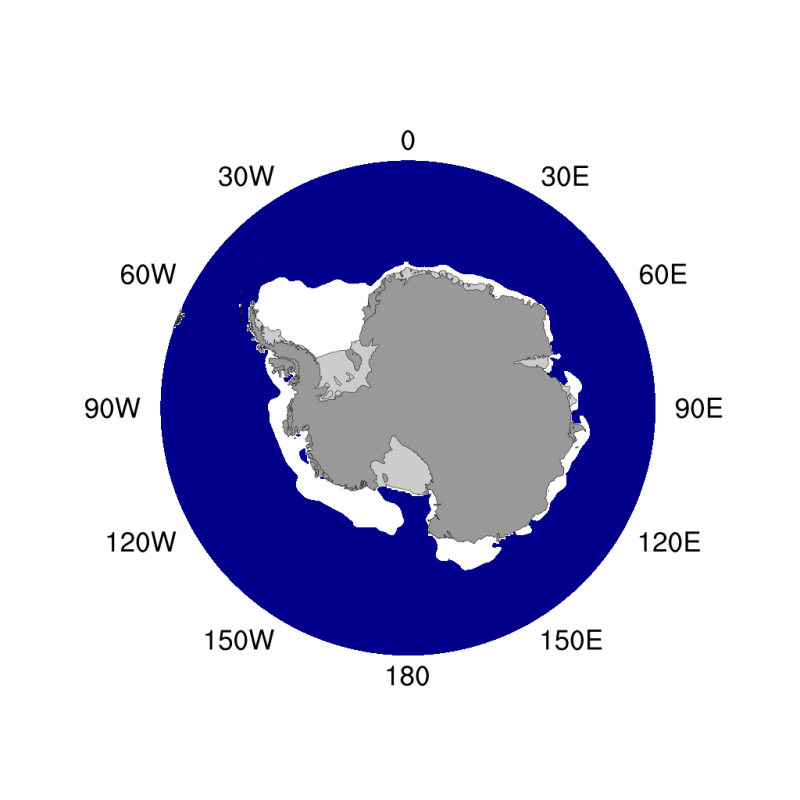
The data sets include four sets of data obtained from the Scanning Multi-channel Microwave Radiometer (SMMR), Special Sensor Microwave Imager (SSM/I) and the Special Sensor Microwave Imager Sounder (SSMIS) sensors using passive microwave remote sensing inversion. SMMR was aboard the Nimbus-7 satellite, and its working period was from October 26, 1978 to July 8, 1987. Since July 1987, the data provided by the SSM/I and the SSMIS aboard the US Defense Meteorological Satellite Program (DMSP) satellite group have been used. The first three data sets contain sea ice concentration data, covering the Antarctic region with a spatial resolution of 25 km: (1) The data were obtained from Nimbus-7 SMMR and DMSP SSM/I-SSMIS Version 1 by applying the NASA Team algorithm inversion. The temporal coverage is from November 1978 to February 2017, with a temporal resolution of one month. A bin file is stored every month. (2) The data source is the same as the first set. The temporal coverage is from 1978-10-26 to 2017-2-28. The temporal resolution is two days, and the spatial resolution is 25 km. A folder was stored every year, and a bin file was stored every other day. (3) The data were obtained from near-real-time DMSP SSMIS by applying the NASA Team algorithm inversion. The temporal coverage is from 2015-1-1 to 2018-2-3, and the temporal resolution is one day. A bin file is stored every day. Each file consists of a 300-byte file title (data time information, projection pattern, file name) and a 316*332 matrix. The fourth set of data is the sea ice coverage and sea ice area time series. The temporal coverage is from November 1978 to December 2017. This data set is a time series sequence of sea ice coverage and sea ice area in the Antarctic. The temporal resolution is one month, and an ASCII file is stored every month. Each file consists of a file title (time, data type), a 39*1 sea ice cover matrix and a 39*1 sea ice area matrix. For further details on the data, please visit the US Ice and Snow Data Center NSIDC website - Data Description http://nsidc.org/data/NSIDC-0051; http://nsidc.org/data/NSIDC-0081; http://nsidc.org/data/G02135
2022-11-02 View Details
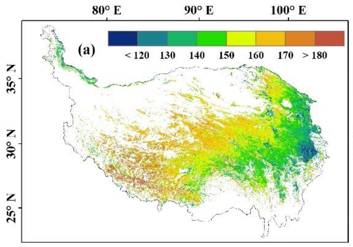
This phenological data is based on the MOD13A2 data of the Qinghai Tibet Plateau from 2000 to 2015 (with a temporal resolution of 16 days and a spatial resolution of 1km). The NDVI curve is fitted using the segmented Gaussian function in the TIMESAT software. The spring phenology, autumn phenology and the length of the growth season are extracted using the dynamic threshold method. The thresholds of spring phenology and autumn phenology are set to 0.2 and 0.7 respectively. The phenological data were masked. Among them, the mask rules are: 1) The maximum value of NDVI must be met between June and September; 2) The average value of NDVI from June to September shall not be less than 0.2; 3) The average NDVI in winter shall not exceed 0.3.
2022-10-24 View Details
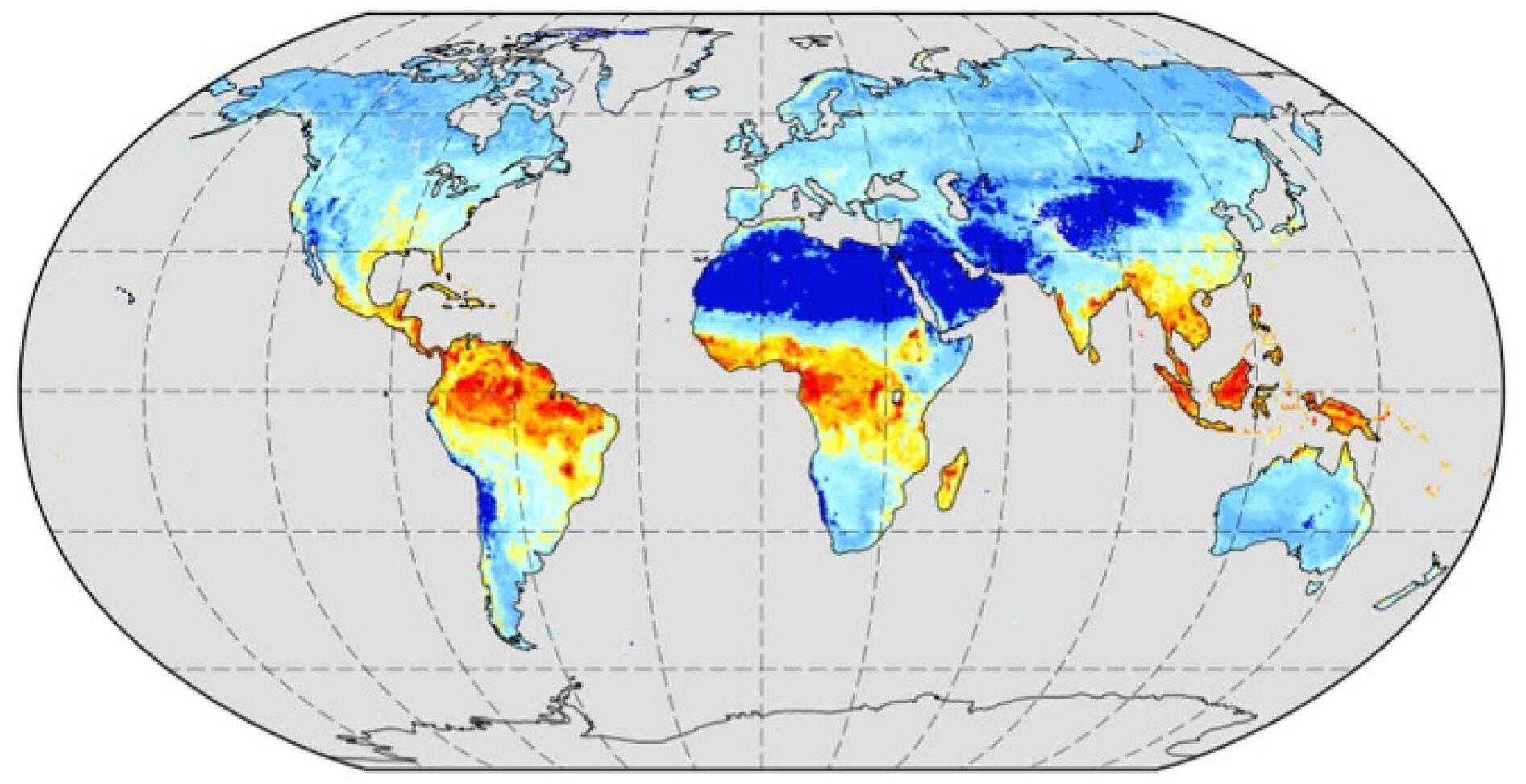
This data set is the global vegetation productivity data, including total primary productivity (GPP), net primary productivity (NPP) and net ecosystem productivity (NEP). It is simulated by BCC-ESM1 model in Phase 6 of the Coupling Model Comparison Plan (CMIP6) under the historical scenario. The data time range is 1850-2014, the time resolution is month, and the spatial resolution is about 2.8125 °. Analog Data Details Visible Link https://www.wdc-climate.de/ui/cmip6?input=CMIP6.CMIP.BCC.BCC -ESM1。
2022-10-24 View Details

This dataset is the daily vorticity related flux observation data of Naqu flux station (31.64 ° N 92.01 ° E, 4598 m a.s.l.), including net ecosystem productivity (NEP), total primary productivity (GPP), ecosystem respiration (ER), evapotranspiration, latent heat, sensible heat, air temperature, relative humidity, wind speed, soil temperature, soil moisture and other data. The main steps of data pre-processing include wild point removal (± 3 σ)、 Coordinate axis rotation (3D wind rotation), Webb Pearman Leuning correction, outlier elimination, carbon flux interpolation and decomposition, etc. Missing data are interpolated through the nonlinear empirical formula between CO2 flux value (Fc) and environmental factors.
2022-10-21 View Details
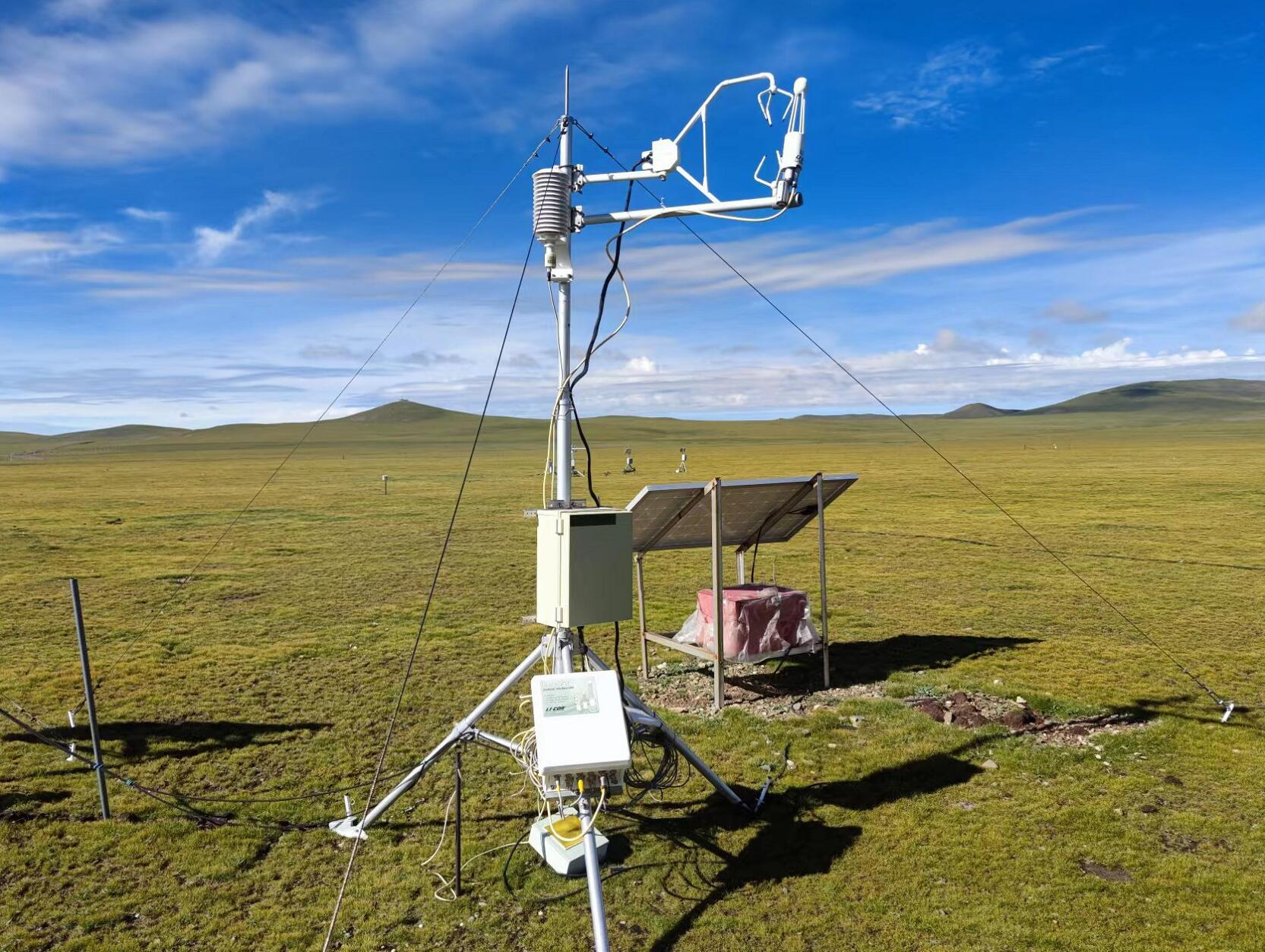
This data set is the daily vorticity related flux observation data of Naqu flux station (31.64 ° N 92.01 ° E, 4598 m a.s.l.), including ecosystem net ecosystem productivity (NEP), total primary productivity (GPP) and ecosystem respiration (ER) data. The main steps of data pre-processing include wild point removal (± 3 σ)、 Coordinate axis rotation (3D wind rotation), Webb Pearman Leuning correction, outlier elimination, carbon flux interpolation and decomposition, etc. Missing data are interpolated through the nonlinear empirical formula between CO2 flux value (Fc) and environmental factors.
2022-10-21 View Details

This dataset is global respiration data, including autotrophic respiration (ra) and heterotrophic respiration (rh). It is simulated by TaiESM1 model in Phase 6 of the Coupling Model Comparison Plan (CMIP6) under historical scenarios. The data time range is 1850-2014, the time resolution is month, and the spatial resolution is about 0.9 ° x1.25 °. Analog Data Details Visible Link https://www.wdc-climate.de/ui/cmip6?input=CMIP6.CMIP.AS -RCEC.TaiESM1.historical。
2022-10-20 View Details
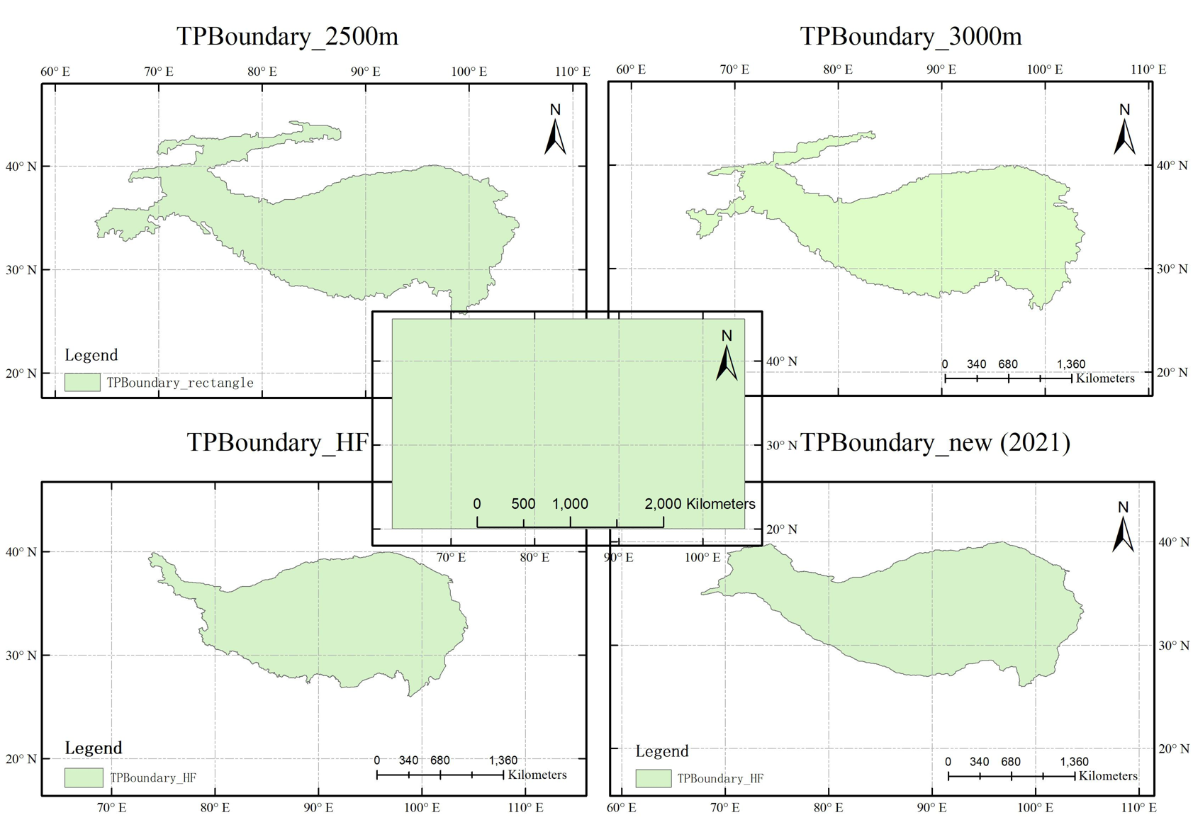
This dataset contains five types of boundaries. 1. TPBoundary_ 2500m: Based on ETOPO5 Global Surface Relief, ENVI+IDL was used to extract data at an elevation of 2500m within the longitude (65~105E) and latitude (20~45N) range in the Tibetan Plateau. 2. TPBoundary_ 3000m: Based on ETOPO5 Global Surface Relief, ENVI+IDL was used to extract data at an elevation of 3000m within the longitude (65~105E) and latitude (20~45N) range in the Tibetan Plateau. 3. TPBoundary_ HF (high_frequency): This boundary is defined according to 2 previous studies. Bingyuan Li (1987) had a systematic discussion on the principles for determining the extent of the Tibetan Plateau and the specific boundaries. From the perspective of the formation and basic characteristics of the Tibetan Plateau, he proposed the basic principles for determining the extent of the Tibetan Plateau based on the geomorphological features, the plateau surface and its altitude, while considering the integrity of the mountain. Yili Zhang (2002) determined the extent and boundaries of the Tibetan Plateau based on the new results of research in related fields and years of field practice. He combined information technology methods to precisely locate and quantitatively analyze the extent and boundary location of the Tibetan Plateau, and concluded that the Tibetan Plateau in China extends from the Pamir Plateau in the west to the Hengduan Mountains in the east, from the southern edge of the Himalayas in the south to the northern side of the Kunlun-Qilian Mountains in the north. On April 14, 2017, the Ministry of Civil Affairs of the People's Republic of China issued the Announcement on Adding Geographical Names for Public Use in the Southern Tibetan Region (First Batch), adding six geographical names in the southern Tibetan region, including Wo’gyainling, Mila Ri, Qoidêngarbo Ri, Mainquka, Bümo La, and Namkapub Ri. 4. TPBoundary_ New (2021): Along with the in-depth research on the Tibetan Plateau, the improvement of multidisciplinary research and understanding inside and outside the plateau, and the progress of geographic big data and Earth observation science and technology, the development of the 2021 version of the Tibetan Plateau boundary data by Yili Zhang and et al. was completed based on the comprehensive analysis of ASTER GDEM and Google Earth remote sensing images. The range boundary starts from the northern foot of the West Kunlun Mountain-Qilian Mountain Range in the north and reaches the southern foot of the Himalayas and other mountain ranges in the south, with a maximum width of 1,560 km from north to south; from the western edge of the Hindu Kush Mountains and the Pamir Plateau in the west to the eastern edge of the Hengduan Mountains and other mountain ranges in the east, with a maximum length of about 3,360 km from east to west; the latitude and longitude range is 25°59′30″N~40°1′0″N, 67°40′37″E~104°40′57″E, with a total area of 3,083,400km2 and an average altitude of about 4,320m. Administratively, the Tibetan Plateau is distributed in nine countries, including China, India, Pakistan, Tajikistan, Afghanistan, Nepal, Bhutan, Myanmar, and Kyrgyzstan. 5. TPBoundary_ Rectangle: The rectangle was drawn according to the range of Lon (63~105E) and Lat (20~45N). The data are in latitude and longitude projection WGS84. As the basic data, the boundary of the Tibetan Plateau can be used as a reference basis for various geological data and scientific research on the Tibetan Plateau.
2022-04-18 View Details
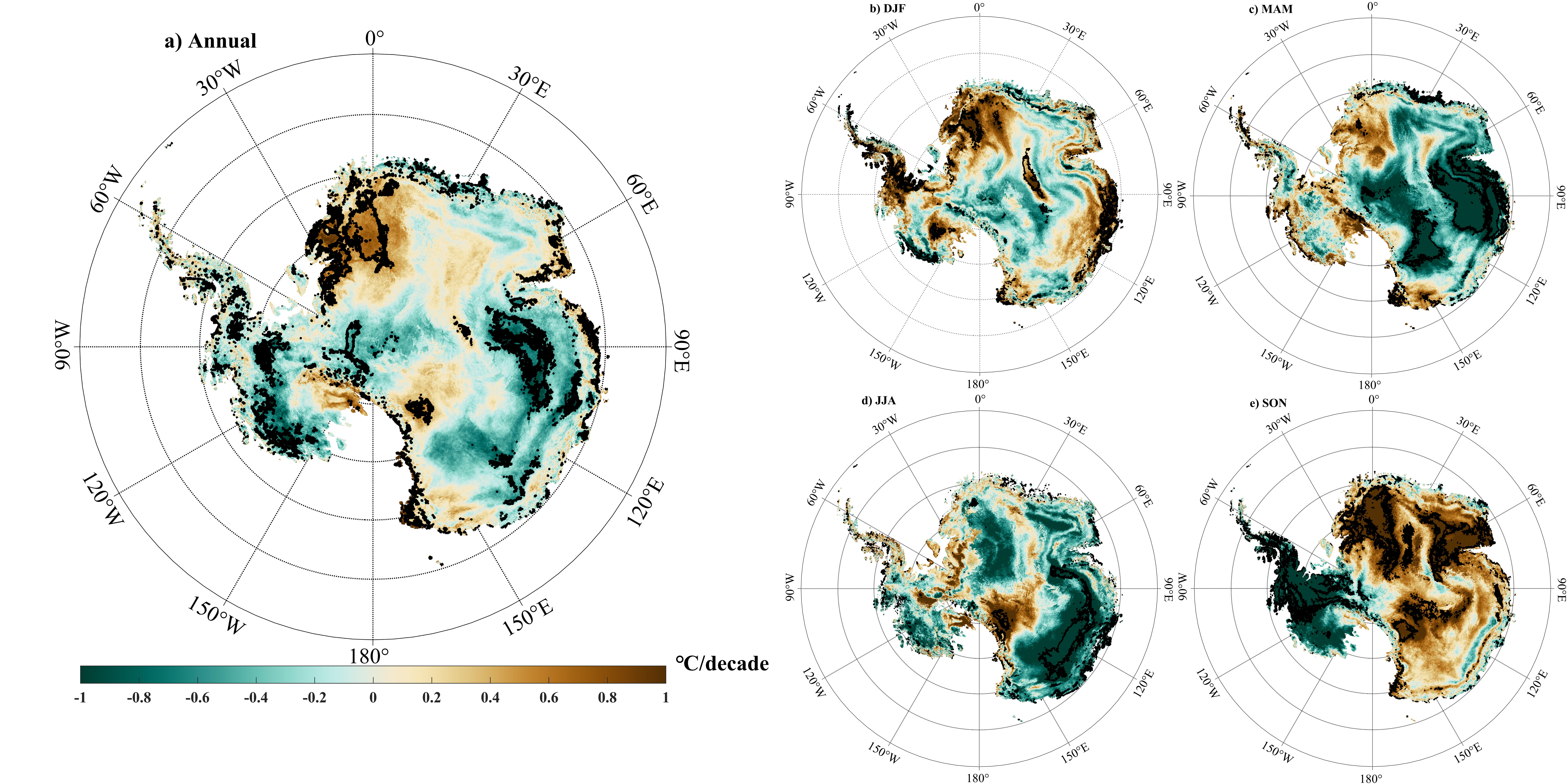
1) Data content: spatial and temporal dataset of near-surface monthly air temperature of Antarctic ice sheet from 2001 to 2018。 2) Data source and processing method: MODIS (MODerate resolution Imaging Spectroradiometer) Land Surface Temperature measurements in combination with in-situ air temperature records from 119 meteorological stations are used to reconstruct a monthly near-surface air temperature product over the Antarctic Ice Sheet (AIS) by means of a neural network model. The product is generated on a regular grid of 0.05°×0.05°, spanning from 2001 to 2018. 3) Data quality description: the accuracy is better than that of ERA5 reanalysis data. 4) Data application achievements and prospects: the database can be used to study the temporal and spatial distribution characteristics of near-surface air temperature of Antarctic ice sheet, and the impact of SAM and ENSO on the interannual variation of Antarctic temperature. In addition, the dataset has the potential application for climate model validation and data assimilation due to the independence of the input of a numerical weather prediction model.
2022-04-15 View Details
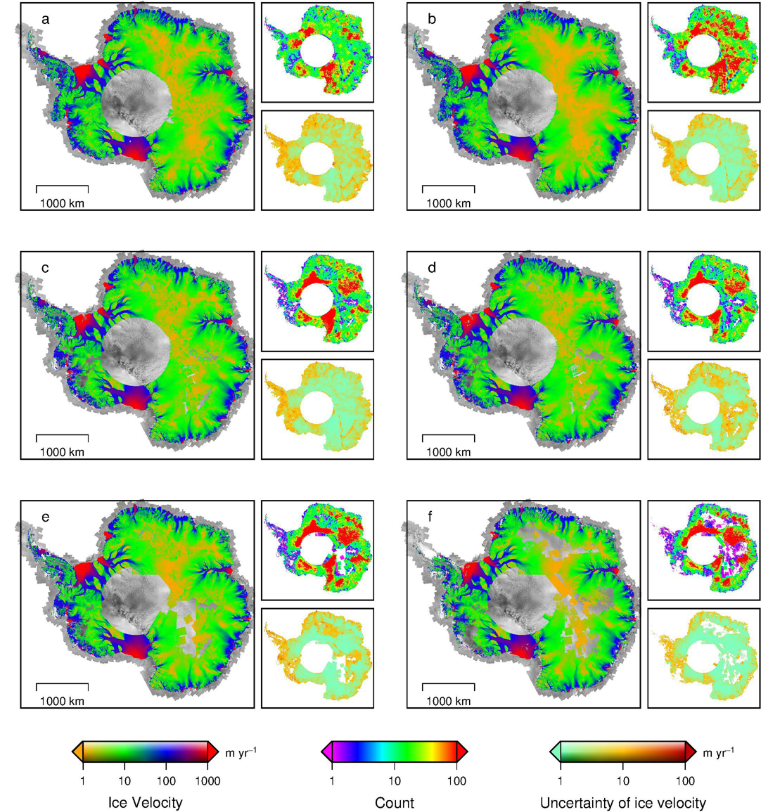
This dataset includes annual mosaics of Antarctic ice velocity derived from Landsat 8 images between December, 2013 and April, 2019, which was updated in 2020 in order to produce multi-year annual ice velocity mosaics and improve the quality of products including non-local means (NLM) filter, and absolute calibration using rock outcrops data. The resulting Version 2 of the mosaics offer reduced local errors, improved spatial resolution as described in the README file.
2022-04-15 View Details
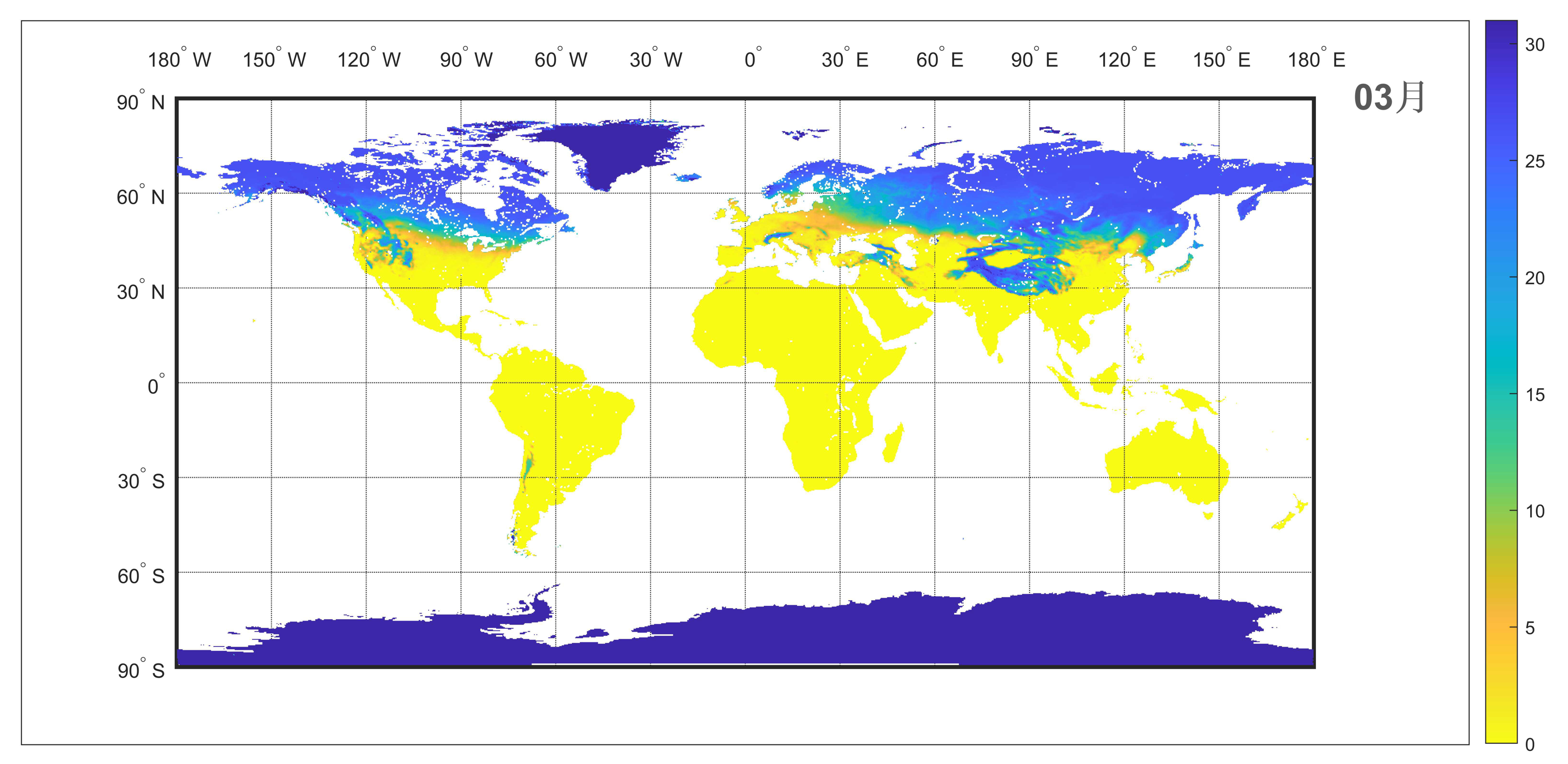
The freeze/thaw status of the near-surface soil is the water-ice phase transition that occurred at the top soil layer. It is an important indicator as a giant on-off “switch” of the land surface processes including water, energy, and carbon exchanges between the land surface and atmosphere. The freeze/thaw status is an essential variable for understanding how the ecosystem responds to and affects global changes. This dataset is based on the AMSR-E and AMSR2 passive microwave brightness temperature data, and the freeze-thaw discriminant function algorithm is used to generate the global near-surface soil freeze-thaw status with a spatial resolution of grids at 0.25° from 2002 to 2019. The dataset can be used for the analysis of the spatial distribution and trend changes of global freeze-thaw cycles, such as the freeze/thaw onset dates and duration. It provides data support for understanding the interaction mechanism between the land surface freeze-thaw cycle and the land-atmosphere exchanges under the context of global changes.
2022-03-30 View Details
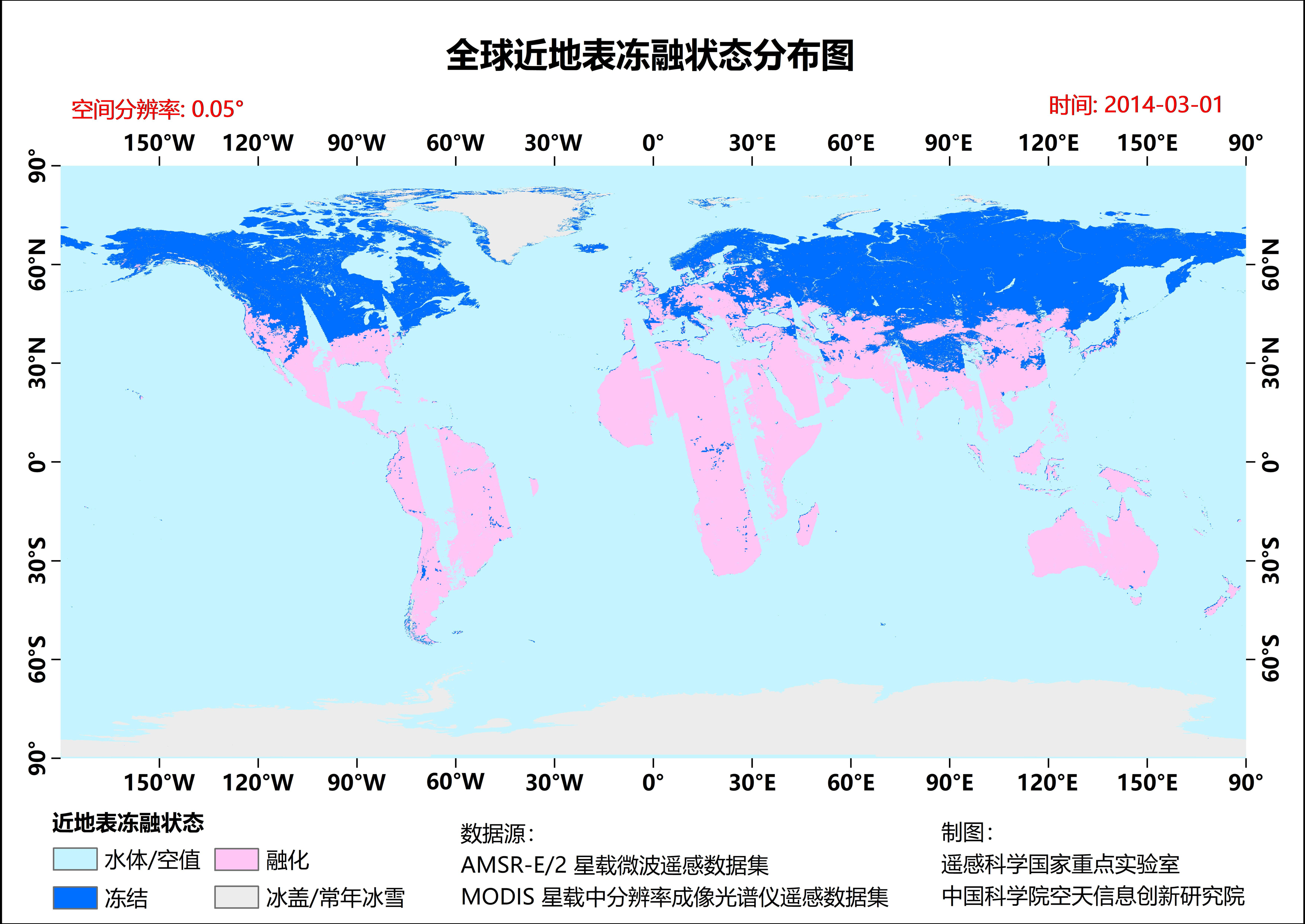
The freeze/thaw status of the near-surface soil is the water-ice phase transition that occurred at the top soil layer. It is an important indicator as a giant on-off “switch” of the land surface processes including water, energy, and carbon exchanges between the land surface and atmosphere. The freeze/thaw status is an essential variable for understanding how the ecosystem responds to and affects global changes. This dataset is based on the AMSR-E, AMSR2 passive microwave brightness temperature data and MODIS optical remote sensing data. The freeze-thaw discriminant function algorithm and downscaling algorithm are used to generate the global near-surface soil freeze-thaw status with a spatial resolution of grids at 0.05° from 2002 to 2017. The dataset can be used for the analysis of the spatial distribution and trend changes of global freeze-thaw cycles, such as the freeze/thaw onset dates and duration. It provides data support for understanding the interaction mechanism between the land surface freeze-thaw cycle and the land-atmosphere exchanges under the context of global changes.
2022-03-28 View Details
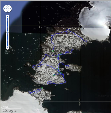
The Antarctic Peninsula is also called "Palmer peninsula" or "Graham land". Located in the southwest polar continent, it is the largest peninsula in the Antarctic continent and the farthest peninsula extending northward into the ocean (63 ° south latitude), bordering the Weddell Sea and berengske sea in the East and West. The Antarctic Peninsula is known as the "tropics" of Antarctica. This is a typical sub polar marine climate. Compared with the Antarctic continent, it is one of the warmest and wettest regions in Antarctica. There are a small number of pioneer plants distributed on the islands in the marginal area, mainly bryophytes and lichens. The spectrum and annotation data of Antarctic Peninsula and its surrounding plants are the spectral data of 37 sample points in 9 regions of Fildes Peninsula and Adeli island around the Antarctic Peninsula on January 7-22, 2018, which provide the background information for the study of the distribution and change of Antarctic plants.
2022-03-28 View Details
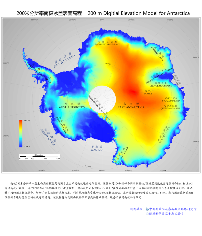
The Antarctic ice sheet elevation data were generated from radar altimeter data (Envisat RA-2) and lidar data (ICESat/GLAS). To improve the accuracy of the ICESat/GLAS data, five different quality control indicators were used to process the GLAS data, filtering out 8.36% unqualified data. These five quality control indicators were used to eliminate satellite location error, atmospheric forward scattering, saturation and cloud effects. At the same time, dry and wet tropospheric, correction, solid tide and extreme tide corrections were performed on the Envisat RA-2 data. For the two different elevation data, an elevation relative correction method based on the geometric intersection of Envisat RA-2 and GLAS data spot footprints was proposed, which was used to analyze the point pairs of GLAS footprints and Envisat RA-2 data center points, establish the correlation between the height difference of these intersection points (GLAS-RA-2) and the roughness of the terrain relief, and perform the relative correction of the Envisat RA-2 data to the point pairs with stable correlation. By analyzing the altimetry density in different areas of the Antarctic ice sheet, the final DEM resolution was determined to be 1000 meters. Considering the differences between the Prydz Bay and the inland regions of the Antarctic, the Antarctic ice sheet was divided into 16 sections. The best interpolation model and parameters were determined by semivariogram analysis, and the Antarctic ice sheet elevation data with a resolution of 1000 meters were generated by the Kriging interpolation method. The new Antarctic DEM was verified by two kinds of airborne lidar data and GPS data measured by multiple Antarctic expeditions of China. The results showed that the differences between the new DEM and the measured data ranged from 3.21 to 27.84 meters, and the error distribution was closely related to the slope.
2021-11-02 View Details
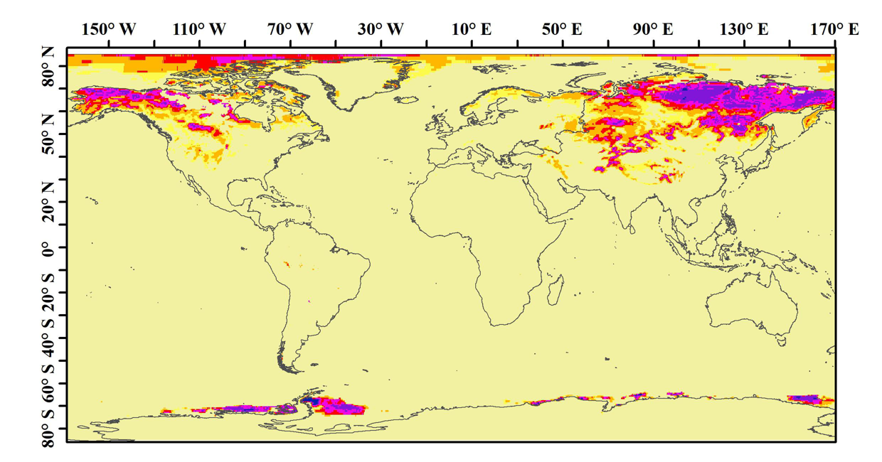
The “Long-term series of daily global snow depth” was produced using the passive microwave remote sensing data. The temporal range is 1980~2018, and the coverage is the global land. The spatial resolutions is 25,067.53 m and the temporal resolution is daily. A dynamic brightness temperature gradient algorithm was used to derive snow depth. In this algorithm, the spatial and temporal variations of snow characteristics were considered and the spatial and seasonal dynamic relationships between the temperature difference between 18 GHz and 36 GHz and the measured snow depth were established. The long-term sequence of satellite-borne passive microwave brightness temperature data used to derive snow depth came from three sensors (SMMR, SSM/I and SSMI/S), and there is a certain system inconsistency among them. So, the inter-sensor calibration was performed to improve the temporal consistency of these brightness temperature data before snow depth derivation. The accuracy analysis shows that the relative deviation of Eurasia snow depth data is within 30%. The data are stored as a txt file every day, each file is a 1383*586 snow depth matrix, and each snow depth represents a 25,067.53m* 25,067.53m grid. The projection of this data is EASE-Grid, and following is the file header which describes the projection detail. File header: ncols 1383 nrows 586 xllcorner -17334193.54 yllcorner -7344787.75 cellsize 25,067.53 NODATA_value -1
2021-08-14 View Details
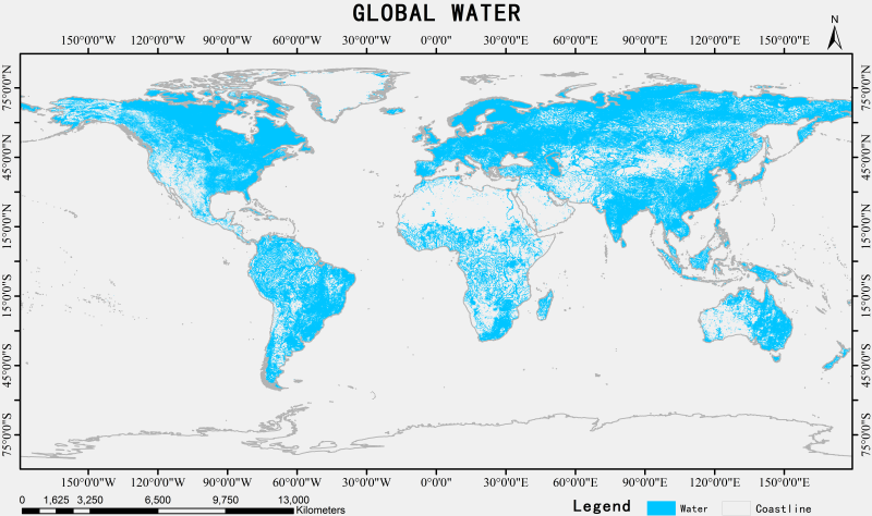
River and lake resources are important components for studying the Earth ecological environment, affecting global ecosystems, heat, material exchange and balance and serving as an important basis for studying changes in the global environmental mechanism. At present, the lack of global lake vector data with large-scale, high-precision, and large-range has hindered hydrological research on rivers and lakes. Taking the data collection of global rivers and lakes of Jun Chen as the source data and combining the domestic high-resolution image GF data of 2 to 3 years before and after 2010, a data set of global rivers and lakes was generated. This data set makes up for the shortcomings of low precision in some areas and is an editable lake and river vector data set with high accuracy.
2020-12-22 View Details
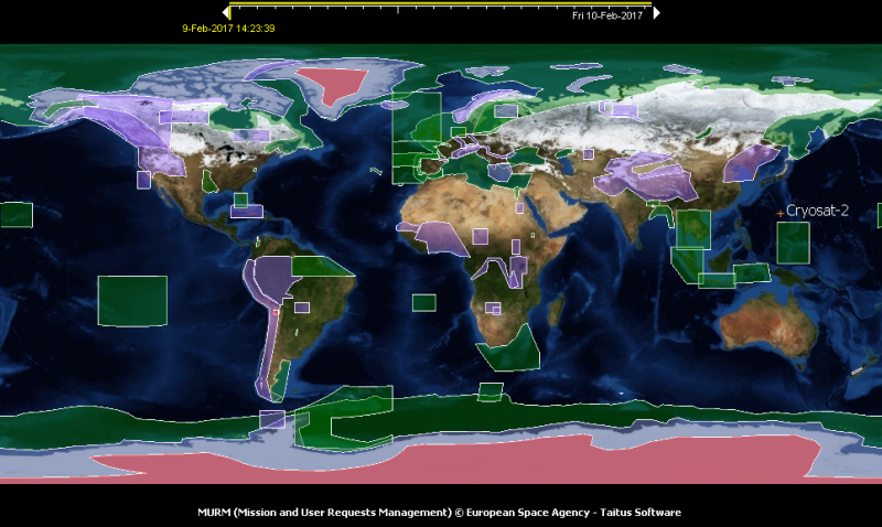
The global Cryosat-2 GDR dataset is generated by the European Space Agency (ESA); it has a temporal coverage from 2010 to 2016 and covers the globe. On April 8, 2010, the ESA launched the Cryosat-2 high-tilt polar orbit satellite. The satellite is equipped with an SAR Interferometer Radar Altimeter (SIRAL), which is mainly used to monitor polar ice thickness and sea ice thickness changes, and, furthermore, to study the effects of melting polar ice on global sea level rise and that of global climate change on Antarctic ice thickness. The altimeter operates in the Ku-band and at a frequency of 13.575 GHz, it includes three measurement modes. One is a low-resolution altimeter measurement mode (LRM) that points to the subsatellite point to obtain all surface observations for land, sea, and ice sheets; its processing is similar to ENVISAT/RA-2, with an orbital resolution of 5 to 7 km. The second is the Synthetic Aperture Radar (SAR) measurement mode, which is mainly used to improve the accuracy and resolution of sea ice observations; it can make the resolution along the orbit reach approximately 250 m. The third is the Interferometric Synthetic Aperture Radar (InSAR), which is mainly used to improve the accuracy of areas with complex terrain such as the edges of ice sheets or ice shelves. The CryoSat -2/SIRAL data products mainly include 0-level data, 1b-level data, 2-level data and high-level data. The Cryosat-2/SIRAL products consist of two files: an XML head file (.HDR) and a data product file (.DBL). The HDR file is an auxiliary ASCII file for fast identification and retrieval of the data files. 1b-level products are stored separately according to the measurement modes, and the data recording formats of different modes are also different. Each waveform in LRM mode and SAR mode has 128 sampling points, while that in SARIn mode has 512 sampling points. 2-level GDR products are available for most scientific applications, including measurement time, geographic location, altitude, and more. In addition, the altitude information in GDR products has been obtained through instrumental calibration, transmission delay corrections, geometric corrections, and geophysical corrections (such as atmospheric corrections and tidal corrections). The GDR products are single global full-track data, that is, the measurement results of the three modes. After different processing, they are combined in chronological order; thereby, the data recording formats are unified. The data in the three modes use different waveform retracking algorithms to obtain altitude values. In the latest updated Baseline C data, the LRM mode data use three algorithms: Refined CFI, UCL and Refined OCOG.
2020-12-17 View Details
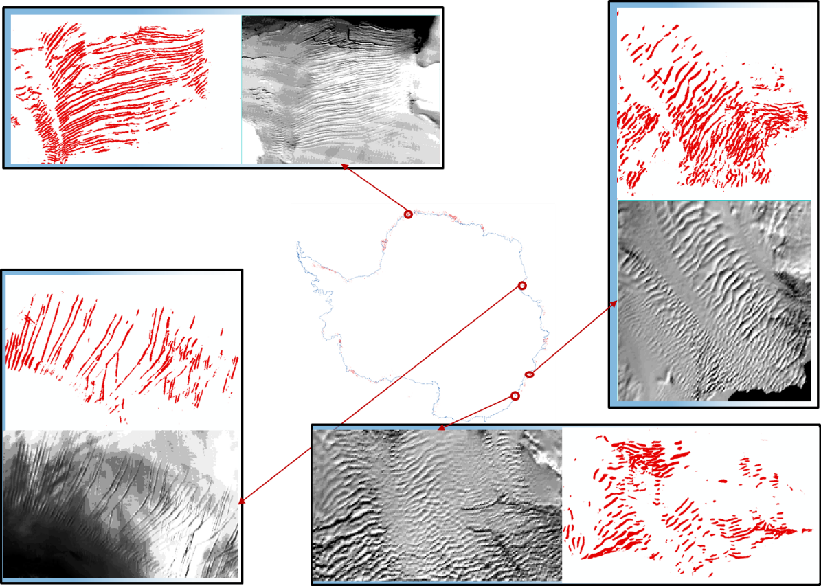
Based on the sentinel-1 hyperspectral wide-band SAR data, using the proposed u-net ice fissure detection method, the ice fissure elevation data of the north and south polar ice sheet are formed. Firstly, the data preprocessing of sentinel-1 hyperspectral wide-band SAR includes radiometric calibration, ice cover range determination and speckle noise removal. In order to suppress the speckle noise of SAR data, and to ensure the ice fracture characteristics, we use ppb method to remove multiplicative noise. This method can not only effectively remove spots, but also retain the characteristics of ice cracks. Secondly, we use the u-net based ice crack detection algorithm to extract ice cracks. In order to obtain the correct ice fracture SAR data samples, we select the SAR samples by comparing the high-resolution optical data of ice fracture to form the ice fracture SAR data samples. Based on the SAR data of ice fracture area and non ice fracture area, we use u-net method to extract ice fracture. Finally, we geocode the detected ice fracture data to form the ice fracture products of the north and south polar.
2020-10-14 View Details
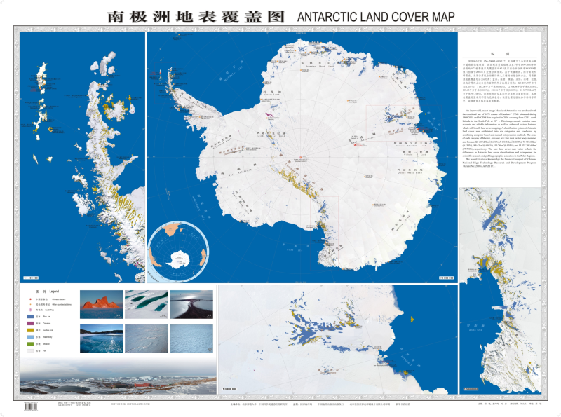
A high-resolution remote sensing image mosaic of the entire Antarctic was generated by synthesizing the 1073 images taken by American Landsat 7 during 1999 to 2003 and the medium-resolution MODIS image (taken in 2005) covering south of 82.5°southern latitude. Based on the mosaic, combined with the needs of Antarctic scientific research, Antarctica land cover was divided into six types using the combination method of computer automatic interpretation and artificial assistance. They were blue ice, fissures, bare rocks, water bodies, moraines and firns, and the areas and proportions of the above types were 225,207.29 square kilometers (1.651%), 7153.36 square kilometers (0.052%), 72,958.04 square kilometers (0.535%), 189.43 square kilometers (0.001%), 310.76 square kilometers (0.003%), and 13337392.66 square kilometers (97.758%), respectively. The map is a satellite image map of approximate true color synthesis, and the regions of various cover types are represented by different color blocks. The map mainly provides a reference for popular scientific research, geography education and science popularization.
2020-10-14 View Details
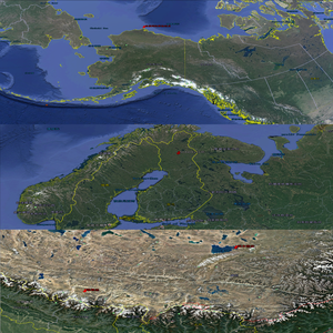
Solar radiation data were obtained using the internationally accepted solar radiation meter (LI200SZ, LI-COR, Inc., USA). The measured data are total solar radiation, including direct and diffuse solar radiation, with a wavelength range of 400-1100 nm. The units of the measurement results are W/㎡, and the typical error under natural lighting is ±3% (within an incident angle of 60°). Data from different locations in the three poles (Everest Station and Namco Station on the Tibetan Plateau, Sodankylä Station in the Arctic, and Dome A Station in the Antarctic) are derived from site cooperation and website downloads. The temporal coverage of data from the Everest Station and Namco Station on the Tibetan Plateau is from 2009 to 2016, that from the Sodankylä Station in the Arctic is from 2001 to 2017, and that from the Dome A Station in the Antarctic is from 2005 to 2014.
2020-10-14 View Details

From 1000 AD to the present, the concentration of methane in the atmosphere has increased significantly in the ice cores of the Antarctic and Arctic. These data came from the Tasmanian laboratory of Australia, where the high resolution data were obtained by using wet extraction of ice core samples, and the same measurement and calibration procedures were applied to all samples. The results are consistent with the results of internationally renowned ice core greenhouse gas laboratories such as the University of Bern, the University of Copenhagen and the University of Ohio. The physical meaning of each variable: First column: time; second column: methane concentration value
2020-10-14 View Details
Contact Support
Links
National Tibetan Plateau Data CenterFollow Us

A Big Earth Data Platform for Three Poles © 2018-2020 No.05000491 | All Rights Reserved
|  No.11010502040845
Tech Support: westdc.cn